The studio

bt.studio(scene) serves a 3D workbench for the scene on 127.0.0.1 and opens your browser. The studio and your Python session hold the same scene: drag the TCP gizmo and IK runs live with the result visible from Python; call scene.set_tcp_target(...) and the browser's robot moves. Everything the UI does, the API does — the two are one operation model over one wire protocol.

bt.studio(scene)                          # blocks until Ctrl-C
server = bt.studio(scene, block=False)    # keep the prompt (REPL / notebook)
server.url
server.stop()

A studio that opens after a headless bake replays it: the demos bake the cycle, write the USD, and only then open the studio with --studio, and the dock has the cycle to play. It is the last bake that is replayed, so a script that bakes more afterwards — a scenario matrix for the report, a sweep — names the one to show:

tl = scene.simulate_sequence("cycle")
runs = scene.simulate_scenarios(["cycle"])   # the FAT rows; the last is now "latest"
scene.show_timeline(tl)                      # the nominal cycle again
bt.studio(scene)

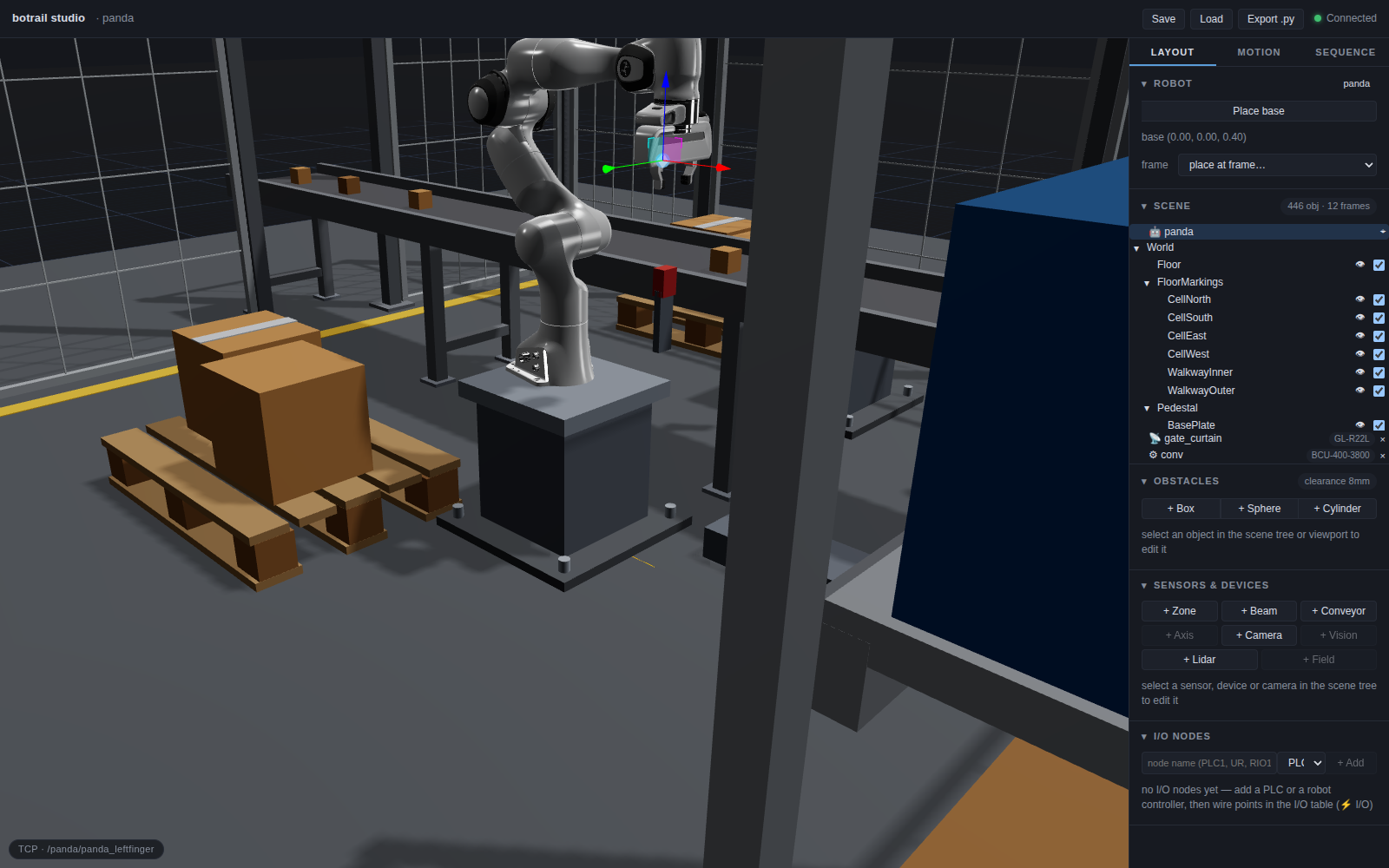
The header names the robot (a dropdown when several share the scene, driving every panel), holds the project buttons — Save / Load are .botrail projects, Export .py is generate_python() — and shows the connection dot. The viewport is a full orbit camera over the cell, with the TCP gizmo on the end-effector and the active TCP link named in the corner badge.

The sidebar is three workflow tabs. LAYOUT builds the world: robot placement, the scene tree, obstacles, sensors & devices. MOTION poses and teaches the selected robot: TCP, joints, waypoints — the things used together. SEQUENCE programs the cell and runs it. Sections collapse from their headers, and the studio remembers the open tab and the sections you keep closed. Picking in the viewport follows along — clicking an arm raises MOTION, clicking an obstacle raises LAYOUT — except while SEQUENCE is up, since picking a part or an arm there is how grasp steps are authored.

Placing the robot — ROBOT

The base pose, editable two ways: Place base for dragging it, or the place at frame dropdown to snap it onto any named frame — the studio form of scene.set_robot_base_pose(*scene.frame(...)).

The cell inventory — SCENE

The scene tree: robots, then the world's obstacles as imported (the counter reads e.g. 147 obj · 5 frames), then sensors and devices. The tree is the list — click an obstacle (here or in the viewport), a sensor, or a device and its editor opens in the section below, inspector style. Colliding obstacles read red right in the tree. Per obstacle, the eye toggles display and the checkbox includes/excludes it from collision checking (set_obstacle_enabled); removal sits in the editor form (and on sensor/device rows).

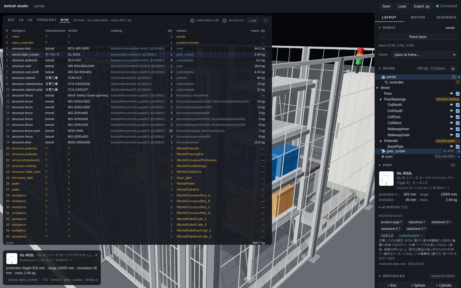
Every row that is a line of the bill of materials wears what it is: the model badge on a catalog arm (UR5e), on the tool welded to it and the controller it needs — two rows under the arm, since the bill names them (arm/tool, arm/controller) though nothing in the scene draws them — on a generated conveyor, a pinned group, an I/O node. The badges are read off scene.bom() as the host derives it, never guessed from the tree, so they cannot disagree with the exported BOM; a line nobody has identified yet wears an amber ? — the rows bom.unidentified() lists, the purchasing to-do read at a glance. The chip at the bottom-left of the viewport names the selection's product too (obstacle · conv/belt · botrail BCU-400-3800), through the group a clicked prim belongs to.

What it is — PART

Under the tree, PART is the line of the bill behind whatever is selected — a robot, an object or the group it sits in, a sensor, a device, a camera, a scanner, an I/O node, one of the derived rows — read off scene.bom(): model and maker, the catalog reference (universal_robots/ur/ur5e/r2 @1d6bfc1; click copies it, ↗ opens the product in the catalog viewer), quantity and purchase unit, and the specs the cell would ask of that kind of line first (payload and reach of an arm, stroke of a gripper, length, width, speed and load of a conveyor), with every attribute a fold away. A catalog arm's card lists its stack — the tool welded on, the controller it needs or the control box its set includes — each a card of its own; a prim inside a pinned group reads one of 12 — fence/east. A line nobody has identified says so, with the scene.set_part(...) that would.

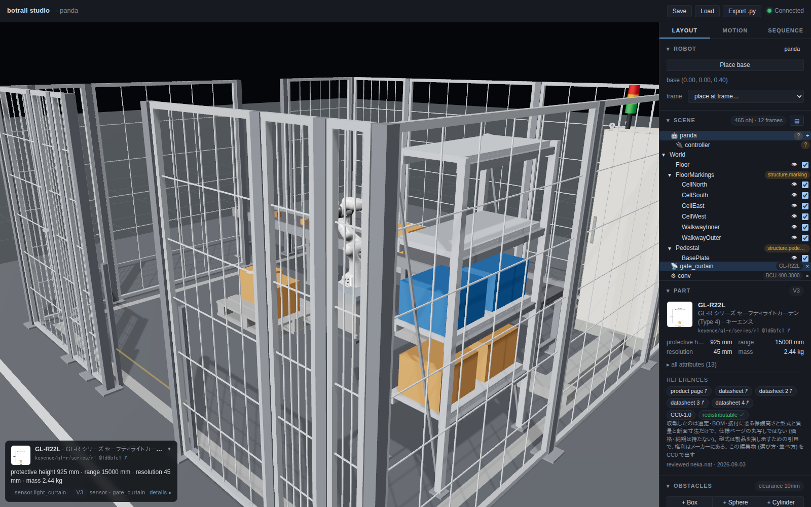
A catalog line has a second layer, read from the catalog itself at the dataset revision the cell resolved the package at — the same bytes the cell was taught on: the product's picture (a spec pack shows its plan), the maker's page, the datasheets and repositories the package was built from, the licence of each set of files and whether they may be redistributed, with the maker's note where there is one (a CAD disclaimer lives nowhere else), the validation level (V2) and who reviewed it, and — for a reference model — what its geometry is and is not. The hub is read once per product and never waited for: with no network the card is the scene's part alone, and ↻ tries again. A package built locally (Robot.from_package) has nothing on the hub to read.

The same card sits in the viewport: the chip at the bottom-left opens into a focus card with the selection's name, reference and headline specs and a details ▸ to this section — so a click on the arm, which raises MOTION, still says what the arm is. Fold it with ▾ or Esc; the studio remembers which shape you keep. Resting the pointer on a body names it beside the cursor (sensor · gate_curtain · KEYENCE GL-R22L), through the group a prim belongs to, and never over what is already selected.

Posing — TCP and JOINTS

The TCP panel picks the IK link (the dropdown defaults to the model's TCP link — on the Franka that is a fingertip, so pick the hand link for grasp work) and switches the gizmo between Move and Rotate. Dragging solves IK continuously; collision turns the offending geometry red as you go. The JOINTS panel is the other door into the same state: one slider per joint.

Teaching motions — MOTION

The panel lists every motion in the scene — Python-authored ones included — with owner and waypoint count. Pick one to edit it (picking another robot's motion also switches the robot, so waypoints always fit), or + new motion to start another; it is created the moment its first waypoint lands. The × at the end of a motion's row deletes it, name and all (remove_motion) — a sequence step that still starts it says so when the cell is checked. Below sits the waypoint-segment editor, mirroring add_segment: pose the robot, then + Joint or + Line appends a segment ending at this configuration (upright adds the orientation-cone constraint that keeps the tool vertical). Plan motion solves the whole list rest-to-rest and plays the preview in the timeline dock, with a tick at each segment boundary:

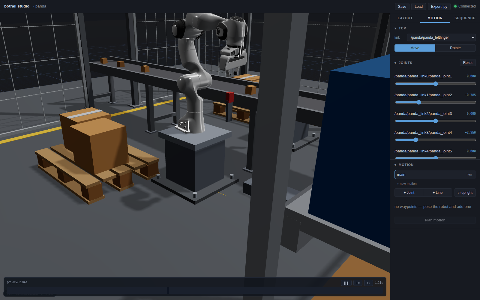
The green readout is the plan: duration, segment count, planning time. A quick A→B check is a one-waypoint motion — pose the goal, + Joint, Plan motion. Trajectories planned from Python against a live session (plan_to_pose) preview in the same dock.

The process — SEQUENCE and RUN

Steps accumulate here the way sq.step(...) writes them: add a motion step from a named motion, a one-second timer step, a grasp/release step for the selected obstacle. The RUN section below holds everything about the next run: with several programs authored (one per station, PLC style), its checkboxes pick which roll together; the dropdown picks the world — baseline or a Python-authored scenario delta (add_scenario); the cap beside the button is the bake's time limit in seconds (the engine's 120 s by default — raise it for a longer cycle; a run still waiting past it comes back as timed out, which is also how a stall under a fault scenario surfaces); Simulate bakes the cycle and broadcasts the timeline to the dock:

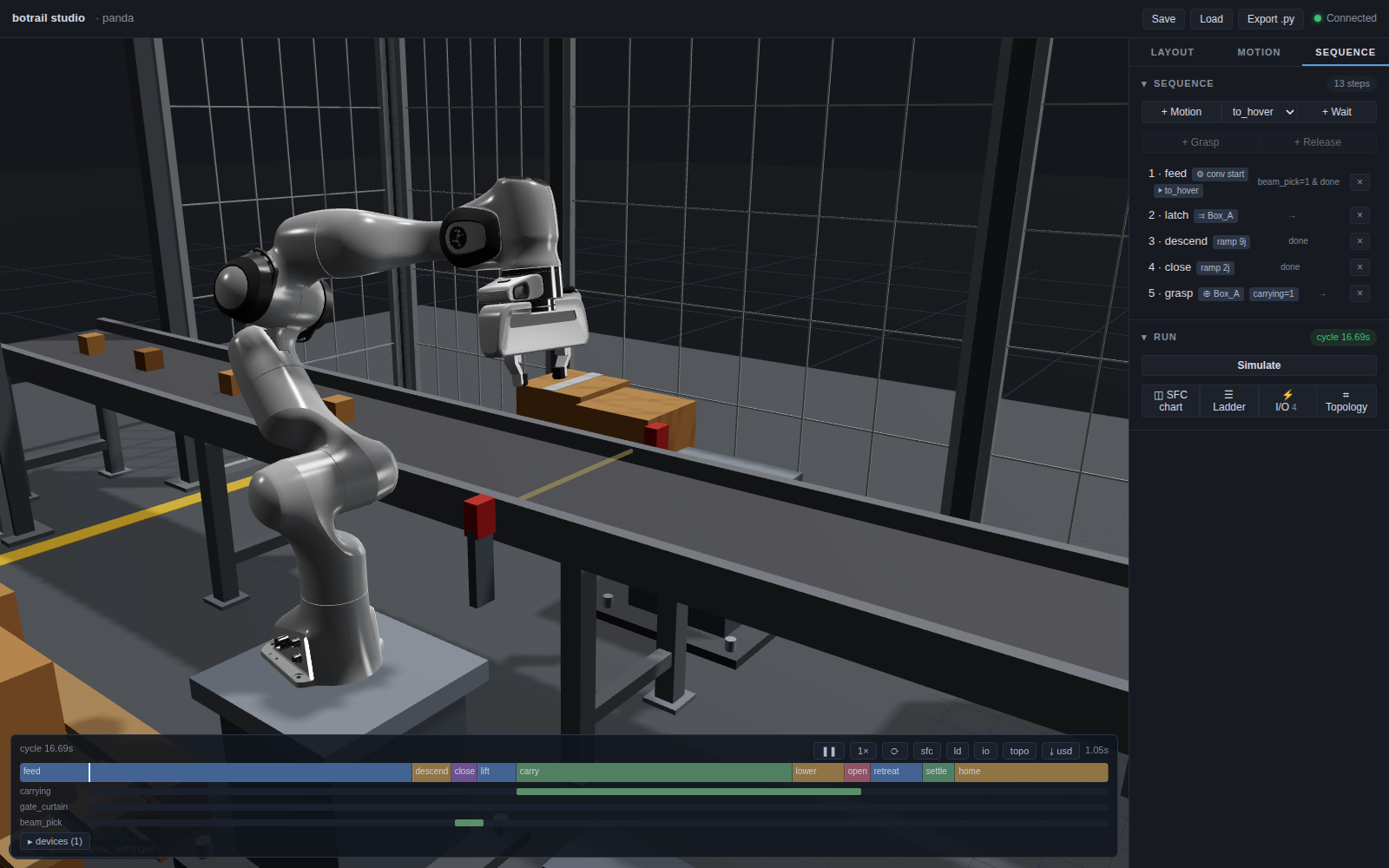
⚛ physics (beside Simulate, and on the dock) is the physics toggle. On, the same bake runs again under the host's physics — the whole cell: every obstacle a rigid body unless it is bolted down, every robot an articulated body, a ground plane at z = 0 — and playback restarts from the top; off, it runs again kinematically and restarts. A physics bake streams: the host sends the tracks as they grow and playback follows, the step bands drawing themselves as the programs advance, so a slow or long bake is watched rather than waited for. When the programs end, the world runs on live from where they left it, in step with the clock — the dock reads cycle 3.00s · world 8.25s — until you switch the toggle off, which stops it and bakes the programs kinematically again; the bake kept for export is the programs' alone. The live world is watched, not kept: neither the host nor the studio records it, so it can run for as long as you like — to see it again, run it again. With no program baked yet, on streams the world under gravity the same way, live from the start: whatever is unsupported falls while an unpowered machine folds. Once playback reaches the live part, a body can be taken in hand — press on a crate, a part, the wall of a tote, a link of a folded arm and drag: a spring pulls the whole body after the mouse (amber line and dot; red when the body is bolted down and cannot move) until you let go. A click on the dock's bar before the live part pauses there to review what happened, and the hand is off while you do; a click on the live part, or ▶, follows the live world again. The world with no program runs until you switch the toggle off, which stops it where it stands; nothing of it is kept to replay or export. Switching on again starts a fresh stream from the cell as authored. What "on" means is the host's choice: bt.studio(scene, physics=bt.Physics(world=True, powered=False)) makes it a power cut, physics=False serves the studio without physics (the toggle says so). The label on the dock names the engine the playing bake ran under; the browser-only session has no thread to stream from and bakes in one go (a fixed ten seconds for the world with no program).

The chart — SFC

◫ SFC chart (in RUN, or the sfc button on the dock) overlays the programs on the viewport in the notation PLC programmers already read — and everyone else reads as a flowchart: one column per program, step boxes joined by transition bars with the condition beside each, a ◇ step fanning into one lane per arm and rejoining below. After a Simulate the chart is the bake's story: steps that ran are outlined, arms the world never took are dashed out, and the guard that won is green — so a scenario that flips a verdict shows up as the other arm lighting up on the next Simulate.

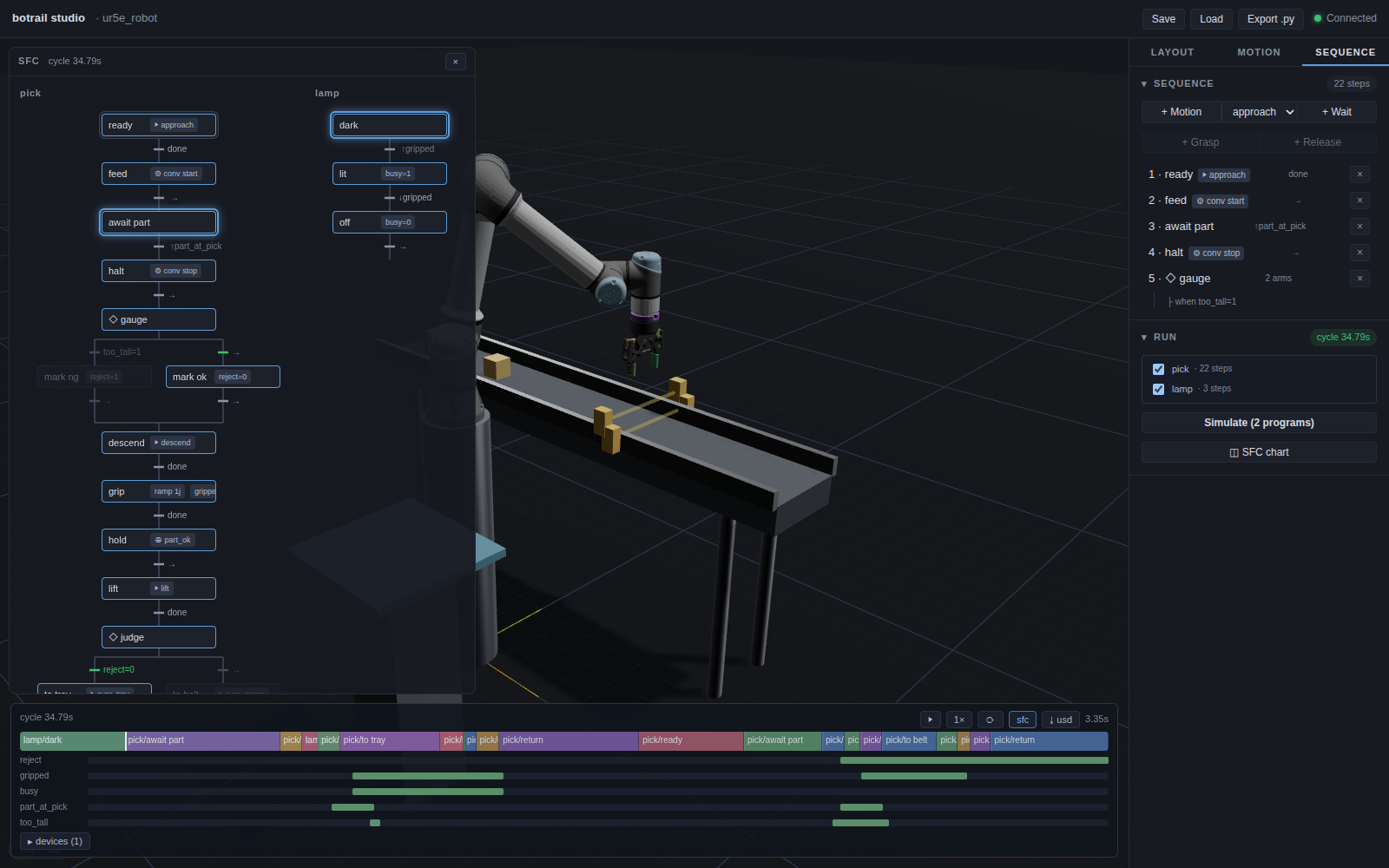
During playback a token rides each program's active step, and the live condition beside it answers why is it waiting: each contact turns green as it becomes true, timers count up (0.29/5.00s), and edge conditions (↑part_at_pick) underline while the signal is high. Just after the token hops, the condition that released it keeps glowing at the old spot for a beat, so the cause of every transition stays readable at playback speed. Clicking any baked step seeks the transport to the moment it began; the chart stays up across reloads until closed.

The chart, the ladder, the I/O table, the topology and the bill of materials below are five views of one panel over the viewport — each is wide, and stacked they hid each other — so opening one closes the others, and the panel's tab strip (SFC · LD · I/O · TOPOLOGY · BOM) switches between them.

The ladder — ☰ LD

☰ Ladder (in RUN, or the ld button on the dock) is the same programs as the SET/RST step ladder a PLC engineer would write them into: one internal relay per step (S0, S1, …, each rung group under its S3 · pick comment), one rung per transition — the step's contact in series with its condition network, ending in (S) the next step and (R) itself — entry actions as output rungs, and elapsed waits as TON timers driven by the step relay. Signals are NO/NC contacts, edges |P|/|N| contacts, all_of/any_of series/parallel contact networks; a ◇ selection becomes one rung per guard, and rung order is its priority — the scan-order first-wins the rollout implements.

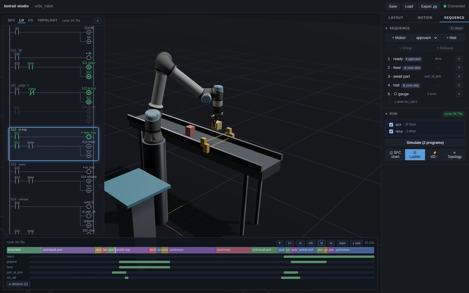
After a Simulate the ladder is a monitor mode: the token frames the active step's whole rung group — comment row down to its last rung, so the box says exactly which rungs the step owns — contacts light green while they conduct at the playhead, TON blocks count up in place (1.47/2.00s), and the instant a transition fires its SET/RST coils flash — while the rungs of arms the bake never took stay dimmed. Clicking a step's comment row seeks the transport to the moment that step became active.

The I/O table — ⚡ I/O

⚡ I/O (in RUN, or the io button on the dock) overlays the I/O map the programs derive: one row per point — direction, kind, the rule that produced it, its host, the channel it is bound to (UR.DI2 · %IX0.2 once bound), tag, status, the steps that write and wait on it — and, while a bake is loaded, the live level of the lane behind it at the playhead. The report's findings sit under the table; unbound filters to what still needs a channel, and the magazine rows (cosmetic) stay folded. Clicking a sensor or device row selects it in the scene tree. The assignment layer is edited here: the channel cell is a select over the channels the point's host (and the stations uplinked to it) offer — used ones named and greyed — auto-assign gives every unbound point the first free compatible channel, and the footer declares and undeclares points (role, kind, safety, pair). Nodes are made in Layout: the I/O nodes inspector adds a PLC / robot controller / remote I/O / safety PLC, and for the node selected in the tree edits its robots, programs, uplink and model, and its channel table through templates (+ DI×8 … + UR standard, with a base address that counts up). Every edit is one message the server validates the way the Python API does, and generate_python writes it all back as add_io_node / bind_input / declare_io.

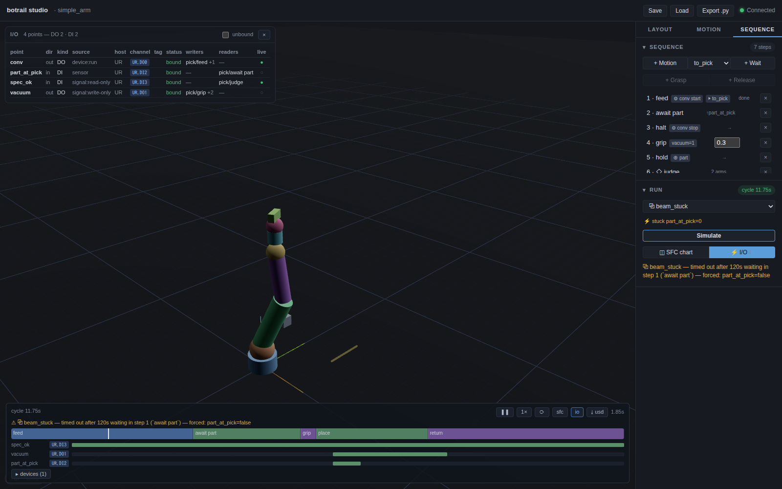
The scene tree lists the I/O nodes (🔌 UR · robot controller, with bound / declared channel counts); selecting one opens a read-only inspector in Layout — kind, programs, robots, uplink, and the channel table with the point on each channel. In RUN, choosing a scenario shows what it changes; a scenario with faults (bt.io.stuck, bt.io.open) lists them, and a run under it that stalls is that scenario's answer, not a broken cell: the last good bake stays on the dock and the diagnosis — the step that stopped and the forced point — is shown beside it, in the same words simulate_scenarios collects in runs.errors.

The topology — ⌗ Topology

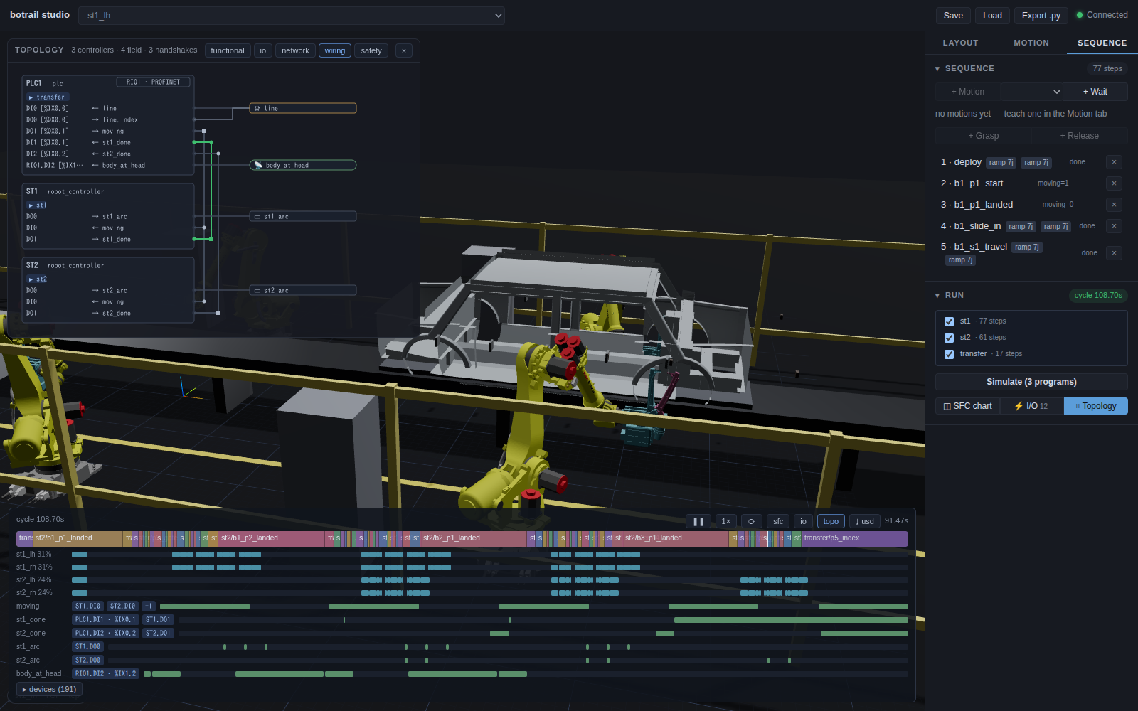
⌗ Topology (in RUN, or topo on the dock) draws the electrical topology over the viewport: one lane per controller — its programs, the stations hanging off it (RIO1 · PROFINET), one row per point with its channel and address — the field side on the right (sensors, devices, robots, field terminals), the wires between them, and the handshake signals between controllers as vertical buses in the gutter, one per signal, a writer tap (■) and a tap (●) per reader. Implicit hosts (<cell>, <robot>) draw dashed; unbound rows and their wires amber and dotted, with a count in the lane header. The layer chips filter the way export_topology(layers=...) does — functional adds program → program routes on the left, io / network / wiring / safety pick the edges — and while a bake plays, every wire with a lane behind it colours green / grey with its live level. Clicking a field node selects it in the scene tree, a lane header selects the node, and a row lights its lane on the dock. The layout is deterministic and never saved: the graph is the one export_topology writes as DOT / Mermaid, so the figure in a design document and this overlay cannot disagree.

The bill — ▤ BOM

▤ on the SCENE section's head (or the BOM tab of the panel) lays the bill of materials over the viewport: every line scene.bom() derives, identified or not, merged by product, in the columns the CSV writes — category, maker, model, catalog reference, quantity, the names it stands for — plus the attributes that have a total, summed in the footer. Lines nobody has identified read amber; unidentified cuts the table to them (the purchasing to-do, bom.unidentified()), derived to the lines nothing in the scene draws (tools, the controller an arm needs). Clicking a row selects what it stands for in the scene tree, and the PART card follows. ⤓ csv downloads the bill as Scene.export_bom writes it — the same bytes.

The timeline dock

The bottom dock is the one transport bar: every playback — a motion preview, a baked cycle, a loaded recording — plays and scrubs here. For a baked sequence it is a timing chart: the cycle time (cycle 16.69s above), one colored band per step, and one lane per signal — internal relays, sensors, device running-states — each lane wearing the channel chip of the point bound to it, so the chart doubles as the addressed I/O waveform sheet. The playback cursor drives the viewport. Recordings loaded with play_usd_animation — including two-robot bakes and Isaac captures — play through the same dock.

A line's bake can carry a hundred lanes, so they never take the viewport over: they scroll inside an area capped at a quarter of the view, and a row of chips — robots, signals, sensors, devices, each with its count — folds a group in or out (device outputs start folded, and sensors do too once a cell has more than twelve). lanes in the dock's header hides them all, leaving the step bar; drag the dock's top edge to size the lane area (double-click it for the default). The browser remembers these choices.

Serving details

bt.studio(scene, host="127.0.0.1", port=0, open_browser=True, block=True)

Use view=((5.9, 4.7, 4.0), (1.25, 0.0, 0.65)) to open at a chosen eye position and orbit target, in world metres. This sets the initial view in the printed/opened browser URL; orbit controls remain interactive, and server.url remains the base endpoint.

port=0 picks a free port. The server binds localhost and serves the bundled UI; in a source checkout build it first (./scripts/build_studio.sh) or point BOTRAIL_STUDIO_DIR at a built studio dist/. Several browsers can connect to one scene — they all see the same state, live. And the studio also runs with no server at all.